Vega-Lite enables concise descriptions of visualizations as a set of encodings that map data fields to the properties of graphical marks.
Altair API kind of works as python wrapper for Vega/Vega-lite library for quickly making statistical visualizations in Python. Actually, the Altair API does not do any visualization rendering per say. All it does is, Altair API creates JSON code/data structure using vega-lite specs such that the JSON data can be visualized by using user-interfaces like Jupyter Lab.
Altair is developed by none other than Jake Vanderplas, the author of Python for Data Science book and Brian Granger, the core contributor of the IPython Notebook and the leader of Project Jupyter Notebook team.
In this post, we will see the basics of getting started with Altair. We will see examples of how to make most commonly used statistical visualizations, like scatter plots, histogram and boxplots and how we can tweak the Altair visualizations to make them look the way want.
Altair Installation
An important thing to remember is that Altair version 2.0 not work with Python 2 and requires Python 3.5 or later.
Here are the steps to install Altair from Jupyter Lab version 0.31,. Both Altair and JupyterLab can be installed with pip:
$ pip install altair==2.0.0rc1
$ pip install jupyterlab
For JupyterLab version 0.31, one needs to additionally run the following:
$ jupyter labextension install @jupyterlab/vega3-extension
On my new Macbook Pro, it threw nodejs error and nodejs needed to be installed first. Altair page has detailed instructions to install.
Getting Started with Altair
Let us just get started plotting with Altair. We will mostly use vega_datasets, a Python package for data sets to make the plots and gapminder data from Software Carpentry website.
import altair as alt
from vega_datasets import data
import pandas as pd
gapminder = data.gapminder()
print(gapminder.head())
   cluster      country  fertility  life_expect       pop  year
0        0  Afghanistan        7.7       30.332   8891209  1955
1        0  Afghanistan        7.7       31.997   9829450  1960
2        0  Afghanistan        7.7       34.020  10997885  1965
3        0  Afghanistan        7.7       36.088  12430623  1970
4        0  Afghanistan        7.7       38.438  14132019  1975
Plotting Scatter Plots with Altair
If you are familiar with ggplot in R, Altair kind of works similar. Altair takes in tidy data and we can add layers of graphics on top of each other with specific rules/functions.
Let us just go ahead and make a scatter plot and understand the code a bit later.
alt.Chart(gapminder).mark_point().encode(
    x='fertility',
    y='life_expect'
)


To make scatter plot (or any plot) with Altair, we will first provide tidy data in the form of Pandas dataframe using Altair’s Chart object like alt.Chart(gapminder). Altair can use the names of the columns efficiently to make visualizations.
To this Chart object, we can further specify what type of visualization we would like. We can map the data to visualization type with an attribute called mark. The mark attribute contains a variety of methods for different type of visualizations. For example, to show the data as points in scatter plots, we need to use mark_point().
We can visualize the Chart(gapminder).mark_point(), but it will show a single point for every row in the data all completely overlapped.
To actually make a scatter plot between x and y-axis, we need to specify which columns in our data should be x and y and which columns we need to use it for attributes like size and color. Altair calls this as encoding variables/columns to different channels and has the method encode(), which
builds a key-value mapping between encoding channels (such as x, y, color, shape, size, etc.) to columns in the dataset, accessed by column name.
By chaining encode method, we can render the scatter plot.
alt.Chart(gapminder).mark_point().encode(
    x='fertility',
    y='life_expect'
)
Since we are using Pandas dataframe for input data, Altair can automatically infer the data types of the variables we are plotting. And also it can appropriately use the variable names for axis names and grid lines.
Plotting Scatter plot with Altair: Changing the Transparency
The above scatter plot example with Altair is one of the basic plots we can make quickly. It looks fantastic for the first try right? However, we often want to tweak and change the looks of scatter plot the way need.
One thing to notice in the above scatter plot is that there are a lot of data points when x-axis values are low. To see the density of the data better, it is a good idea to make the point a bit transparent, so we will know about the overlapping data points.
We can easily change the transparency with opacity argument inside the encode(). Just to repeat, We start giving the data to chart object and then chain mark_point() method to make scatter plot and then chain encode to specify x and y axis. Inside the encode, in addition to x and y-axis, now we also have the argument opacity=alt.value(0.5) to set 50% transparency or opacity.
alt.Chart(gapminder).mark_point().encode(
    x='fertility',
    y='life_expect',
    opacity=alt.value(0.5)
)
With transparency set, now the plot looks definitely better, data points are not clumped as before.

Scatter plot with Altair: changing the color
To change the color of the data points, we specify a color as argument to color inside. In this example, we simply want all the points to be in red, so we specify color=alt.value(‘red’)
alt.Chart(gapminder).mark_point().encode(
    x='fertility',
    y='life_expect',
    opacity=alt.value(0.5),
    color=alt.value('red')
)

Scatter plot Altair: Specifying the data types.
Let us use gapminder data set from Software Carpentry. This data set contains continent information in addition to life expectancy, population, and gdpPercap and will be useful to illustrate a few important aspects of making a good plot.
gapminder = pd.read_csv('gapminder-FiveYearData.csv')
gapminder.head()
Till now, we let Altair infer the types of data on x and y-axis. If we don’t specify data types and use pandas dataframe as input data, by default Altair uses “quantitative” for any numeric data, “temporal” for date/time data, and “nominal” for string/text data.
We can also specify the data types either in long-form or a short-form inside the encode function. Here are the long and short hand notations for specifying the data type, quantitative:Q, ordinal:O, nominal:N, and temporal:T.
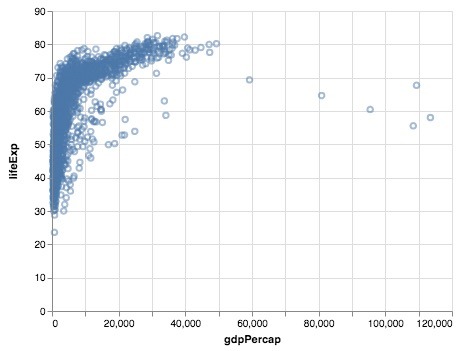
Here is an example of a scatter plot, by specifying the data types in shorthand form.
alt.Chart(gapminder).mark_point().encode(
    x='gdpPercap:Q',
    y='lifeExp:Q',
    opacity=alt.value(0.5)
)
Scatter Plot with Altair: log-transforming x-axis
Often one has to transform one of the axes, like log transformation of x or y-axis. Let use see an example of why and how to do log transformation and make a plot.
If you look at the scatter plot from the above example between gdpPercap and lifeExp, most of the data points are squeezed towards the left side of x-axis. The reason is that there are few points or outliers with large values of gdpPercap.
A better way to visualize this plot is to do the log transformation of the x-axis values. The log transformation will help spread out the x-axis variable values evenly.
We can do the log transformation to x-axis, using alt.X argument inside encode instead of simply specifying x. Inside alt.X, we will specify the variable name followed by scale argument as alt.X(‘gdpPercap:Q’, scale=alt.Scale(type=’log’))
alt.Chart(gapminder).mark_circle().encode(
    alt.X('gdpPercap:Q',
          scale=alt.Scale(type='log')),
    alt.Y('lifeExp:Q',
          scale=alt.Scale(zero=False))
)
Here is how the scatterplot looks like after log-transforming the x-axis. And clearly it looks much better.


Scatter Plot with Altair: coloring the data with a variable
Earlier, we saw an example of coloring data point by specifying a single color we want. Often, we would like to color the data points using one of the variables in the data to see the trend of the data with respect to the variable.
We can easily do that in Altair by specifying the variable name inside encode method, Let us color our scatterplot with continent variable in our dataset.
alt.Chart(gapminder).mark_circle().encode(
    alt.X('gdpPercap:Q',
          scale=alt.Scale(type='log')),
    alt.Y('lifeExp:Q',
          scale=alt.Scale(zero=False)),
     color='continent:N'
)
Altair automatically chooses color and colors data points correspond to each data point based on its continent value. So each continent is colored with a different color.


Plotting Scatter plot with Altair: removing the grid lines
The grid lines on a plot sometimes can be a bit distracting. We can remove the grid lines on x or y-axis by specifying the argument grid=False inside alt.X() or alt.Y() method in the encoding channels. Here is an example code to remove the grid lines from both x and y-axis.
alt.Chart(gapminder).mark_circle(size=50).encode(
    alt.X('gdpPercap:Q', scale=alt.Scale(type='log'),
         axis=alt.Axis(title='GDP Per Capita', grid=False)),
    alt.Y('lifeExp:Q', scale=alt.Scale(zero=False),
         axis=alt.Axis(title='Life Expectancy', grid=False)),
     color='continent:N',
     opacity=alt.value(0.5)
)

alt.Chart(gapminder).mark_circle().encode(
    alt.X('gdpPercap:Q',
           scale=alt.Scale(type='log')),
    alt.Y('lifeExp:Q',
           scale=alt.Scale(zero=False)),
     color='continent:N',
    size='pop:Q'
)


Plotting Histograms with Altair
To plot histograms with Altair, we can use mark_bar() method and chain it to chart object. Note that we need to specify y axis as count with y=’count(*):Q.
alt.Chart(gapminder).mark_bar().encode(
    alt.X("life_expect:Q",
           bin=True),
    y='count(*):Q',
)

Altering bin size in histogram with Altair
Altair, automatically uses a fixed number of bins to make histogram. To change the number of bins, we need to use bin argument inside alt.X() method with bin=alt.BinParams(maxbins=100)
Here is an example with bin size 100.
alt.Chart(gapminder).mark_bar().encode(
    alt.X("life_expect:Q",
          bin=alt.BinParams(maxbins=100)),
    y='count(*):Q'
)

alt.Chart(gapminder).mark_area(
    opacity=0.3,
    ).encode(
      alt.X('lifeExp', bin=alt.Bin(maxbins=100)),
      alt.Y('count(*):Q', stack=None)
)

Boxplots with Altair
Altair does not have a function for making boxplot yet. However, being a declarative language it is easy to build boxplot.
Altair website has an example of boxplot with min/max whiskers. Here is a custom boxplot function with slightly modified code from the altair example.
The boxplot function takes in data, and what variables need to be x and y-axis. It assumes that on x-axis we have a nominal/categorical variable and on y-axis we have a quantitative variable. It also has default size and width of the boxplot, where size refers to the width of the box in boxplot and width refers to the width of the actual plot.
def boxplot_altair(data, x, y, xtype='N', ytype='Q',
                   size=40, width=400):
"""
Python function to make boxplots in Altair
"""
    # Define variables and their types using f-strings in Python
    lower_box=f'q1({y}):{ytype}'
    lower_whisker=f'min({y}):{ytype}'
    upper_box=f'q3({y}):{ytype}'
    upper_whisker=f'max({y}):{ytype}'
    median_whisker=f'median({y}):{ytype}'
    x_data=f'{x}:{xtype}'

    # lower plot
    lower_plot = alt.Chart(data).mark_rule().encode(
        y=alt.Y(lower_whisker, axis=alt.Axis(title=y)),
        y2=lower_box,
        x=x_data
    ).properties(
        width=width)

    # middle plot
    middle_plot = alt.Chart(data).mark_bar(size=size).encode(
        y=lower_box,
        y2=upper_box,
        x=x_data
    ).properties(
        width=width)

    # upper plot
    upper_plot = alt.Chart(data).mark_rule().encode(
        y=upper_whisker,
        y2=upper_box,
        x=x_data
    ).properties(
        width=width)

    # median marker line
    middle_tick = alt.Chart(data).mark_tick(
        color='white',
        size=size
    ).encode(
        y=median_whisker,
        x=x_data,
    )

    # combine all the elements of boxplot to a single chart object
    chart = lower_plot + middle_plot + upper_plot + middle_tick

    # return chart object
    return chart
Let us use the gapminder data to make a few boxplots.
print(gapminder.head())
       country  year         pop continent  lifeExp   gdpPercap
0  Afghanistan  1952   8425333.0      Asia   28.801  779.445314
1  Afghanistan  1957   9240934.0      Asia   30.332  820.853030
2  Afghanistan  1962  10267083.0      Asia   31.997  853.100710
3  Afghanistan  1967  11537966.0      Asia   34.020  836.197138
4  Afghanistan  1972  13079460.0      Asia   36.088  739.981106
Let us make boxplot with continent on x-axis and lifeExp on y-axis with default size and width.
boxplot_altair(gapminder, 'continent', 'lifeExp', width=400)


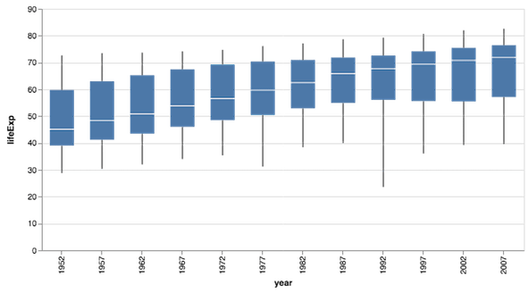
Here is another boxplot with year on x-axis and on y-axis. Here using default size and width will not work. Since the number of categories in the x-axis is large, we need to specify larger width and smaller size.
boxplot_altair(gapminder, 'cluster', 'life_expect',
               size=30, width=600)