tSNE, short for t-Distributed Stochastic Neighbor Embedding is a dimensionality reduction technique that can be very useful for visualizing high-dimensional datasets. tSNE was developed by Laurens van der Maaten and Geoffrey Hinton.
Unlike, PCA, one of the commonly used dimensionality reduction techniques, tSNE is non-linear and probabilistic technique. What this means tSNE can capture non-linaer pattern in the data. Since it is probabilistic, you may not get the same result for the same data.
As Laurens van der Maaten explains on tSNE
“t-SNE has a non-convex objective function. The objective function is minimized using a gradient descent optimization that is initiated randomly. As a result, it is possible that different runs give you different solutions. Notice that it is perfectly fine to run t-SNE a number of times (with the same data and parameters), and to select the visualization with the lowest value of the objective function as your final visualization.”
Let us see an example of using tSNE using Python’s SciKit. Let us load the packages needed for performing tSNE.
import matplotlib.pyplot as plt
import seaborn as sns
%matplotlib inline
import pandas as pd
We will first use digits dataset available in sklearn.datasets.
Let us first load the dataset needed for dimensionality reduction with tSNE.
from sklearn.datasets import load_digits
digits = load_digits()
The digits data contains the classic MNIST data set for pattern recognition of numbers from 0 to 9. In addition to the images, sklearn also has the numerical data ready to use for any dimensionality reduction techniques.
digits.data.shape
We can see that digits.data is a matrix of size (1797, 64). The MNSIT dataset also actual digit for each image/data and it is stored in digits.target
>digits.target

array([0, 1, 2, ..., 8, 9, 8])
Let us subset the data so that we can do the tSNE faster. Her we subset both the data set and the actual digit it correspond to.
data_X = digits.data[:600]
y = digits.target[:600]
tSNE is implemented for us in sklearn. We can call tSNE from sklearn.manifold module. Let us first initialize tSNE and get two components.
from sklearn.manifold import TSNE
tsne = TSNE(n_components=2, random_state=0)
We can then feed our dataset to actually perform dimensionality reduction with tSNE.
tsne_obj= tsne.fit_transform(data_X)
We get a low dimensional representation of our original data in just two dimension. Here it is simply a two dimesional numpy array.
tsne_obj

array([[ 39.19089  , -12.494858 ],
       [-19.107777 ,  -6.754124 ],
       [-16.293173 ,   1.17895  ],
       ...,
       [-21.01011  ,  18.395842 ],
       [  1.2539911, -41.83787  ],
       [  8.800914 ,  -3.2458448]], dtype=float32)
We have actually done the tSNE. Let us make a scatter plot to visualize the low-dimensional representation of the data. Let us store results from tSNE as a Pandas dataframe with the target integer for each data point.
tsne_df = pd.DataFrame({'X':tsne_obj[:,0],
                        'Y':tsne_obj[:,1],
                        'digit':y})
tsne_df.head()


X	Y	digit
0	39.190891	-12.494858	0
1	-19.107777	-6.754124	1
2	-16.293173	1.178950	2
3	21.397039	9.988230	3
4	-34.890625	-3.633268	4
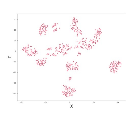
Let us first make a scatter plot with using the two arrays we got from tSNE. We see that the data clusters nicely.
sns.scatterplot(x="X", y="Y",
              data=tsne_df);
Since we also know the identity of each data point, in this case target digit, let us color and label each digit.
sns.scatterplot(x="X", y="Y",
              hue="digit",
              palette=['purple','red','orange','brown','blue',
                       'dodgerblue','green','lightgreen','darkcyan', 'black'],
              legend='full',
              data=tsne_df);
We can clearly see that tSNE nicely captured the patterns in our data. Same digits are mostly in the same cluster.


