


It is a big book and around for a while in ML/DL time scales. I always wanted to check it. Thanks to the review e-copy of the book, finally checked it out. The book has 18 chapters covering all aspects of Machine Learning in the first 12 chapters and basics of Neural Networks and Deep Learning in the last 6 chapters.
So far I could go through and work through most of the early chapters (first six) on Machine Learning. And here are some quick thoughts on the book after going through a few chapters.
What I like About Python Machine Learning?
TLDR: If you are interested in quick summary, go buy it if you are interested in learning ML and Deep Learning. I would highly recommend getting physical copy. I have the soft copy and made it harder for me.
One of the first things that struck me while going through the book is how it stands out from rest (most) of the Machine Learning books. It is a very hands-on book to learn Machine Learning, but the book is not afraid to show some math behind the methods.
And most chapters explaining new technique starts with how to do from scratch and then show how to use the technique from scikit-learn. I think one of the reasons for the stress on the strong foundation plus hands on learning is because the book came out of course-work that Sebastian teaches almost every year.
What can you learn from Python Machine Learning?
If you are keen to know what this book can teach you, here is a really quick outline on some of the chapters covered in the book. Second chapter of the book teaches you “Training Simple Machine Learning Algorithms for Classification”. It starts with implementing one of the most fundamental algorithm in ML for classification, “perceptron” and implements a perceptron from scratch. It is an extremely useful chapter for learning both classic Machine Learning and Deep Learning.
Chapter 3 take you on “A Tour of Machine Learning Classifiers Using scikit-learn”. Here you can learn most commonly used algorithms, and get started with scikit-learn to implement linear classification algorithms in Python. The fourth chapter is all about “data munging” for “Building Good Training Datasets” to build good machine learning models. This is one of the most important chapters that actually teaches you the practical aspect is of doing machine learning. You will learn
- How to removing and impute missing values from the dataset
- How to deal with categorical data to use in machine learning algorithms
- How to select features that are relevant for the machine learning model.
And chapter 5 is all about dimensionality reduction and how you can use them for feature selection. It starts with vanilla “PCA” and teaches you the classic Linear discriminant analysis and goes to non-linear dimensionality reduction technique with kernel principal component analysis (KPCA).
And chapter 6 puts all the things you have learned in chapter upto 5 to use and learn how to build a good machine learning models, fine tune them, and learn to evaluate the models
Perceptron Learning Algorithm in Python from Scratch
The best way to learn from the book is to work through the chapters. By working through the chapters, you will not only learn Machine Learning and also get better in Python as sebastin uses a great mix of NumPy, Pandas, and scikit-learn.
I will definitely doing that. Here is quick example of working through code snippets from the book but on a different data set. Here I work through “Perceptron classifier”, one of the fundamental classification algorithms detailed in Chapter 2.
In the book, Perceptron learning algorithm is illustrated using the classic IRIS data set. Here, instead of Iris dataset we use Palmer penguins dataset . We will see an example of using Perceptron learning algorithm code in Python from the book to build a machine learning model and predict penguin species using two penguin features.
Let us start with loading the packages needed.
import numpy as np
import pandas as pd
import matplotlib.pyplot as plt
import seaborn as sns
We will use palmer penguins dataset available from Seaborn’s built-in datasets.
penguins = sns.load_dataset("penguins")
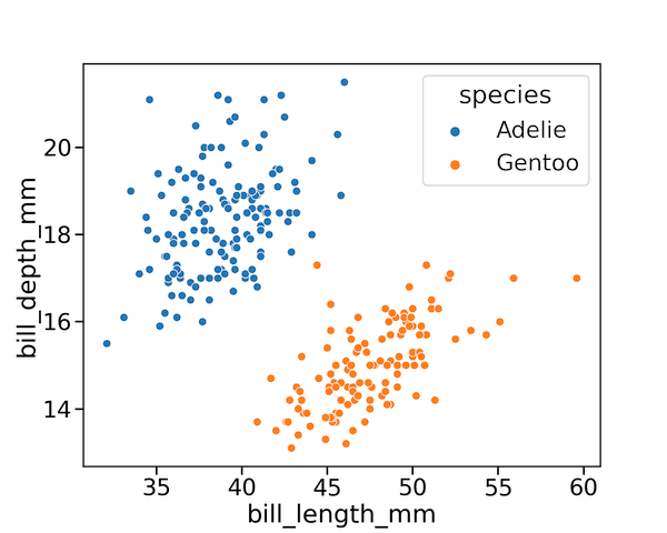
For the sake of simplicity we will only consider two features from the dataset and also remove any observations with missing values. The two features we will use here is Penguins’s bill length and depth. Our class variable is “species” and we will subset the data to contain just two species values.
df = penguins[['species',"bill_length_mm", "bill_depth_mm"]]
df = df.query('species != "Chinstrap"')
df = df.dropna()
And this is how our data looks like.
df.head()

species	bill_length_mm	bill_depth_mm
0	Adelie	39.1	18.7
1	Adelie	39.5	17.4
2	Adelie	40.3	18.0
4	Adelie	36.7	19.3
5	Adelie	39.3	20.6
Let us first visualize the data by simply making a scatter plot and coloring them by species.
sns.set_context("talk", font_scale=1.5)
plt.figure(figsize=(10,8))
sns.scatterplot(x="bill_length_mm",
                #y="flipper_length_mm",
                y="bill_depth_mm",
                hue="species",
                data=df)
plt.savefig("penguin_scatterplot_Seaborn.png",
                    format='png',dpi=150)
We can clearly see that the there is clear separation between the species and will be a great data set for our Perceptron learning algorithm.

We will be using the Perceptron algorithm implemented in Python from scratch. It mainly uses Numpy, therefore let us convert the features and class variables in Pandas data frame into NumPy arrays.
y = df.iloc[:, 0].values
y = np.where(y == 'Adelie', -1, 1)
# extract bill length and depth from the dataframe as arrays
X = df.iloc[:, [1, 2]].values
Perceptron Algorithm
Here is the Python Class implementing Perceptron algorithm from the book. Check out the code repository available for the 3rd edition of the book.
class Perceptron(object):
       """Perceptron classifier.
       Parameters
       ------------
       eta : float
         Learning rate (between 0.0 and 1.0)
       n_iter : int
         Passes over the training dataset.
       random_state : int
         Random number generator seed for random weight
         initialization.
       Attributes
       -----------
       w_ : 1d-array
         Weights after fitting.
       errors_ : list
         Number of misclassifications (updates) in each epoch.
       """
       def __init__(self, eta=0.01, n_iter=50, random_state=1):
           self.eta = eta
           self.n_iter = n_iter
           self.random_state = random_state

       def fit(self, X, y):
           """Fit training data.
           Parameters
           ----------
           X : {array-like}, shape = [n_examples, n_features]
             Training vectors, where n_examples is the number of
             examples and n_features is the number of features.
           y : array-like, shape = [n_examples]
             Target values.
           Returns
           -------
           self : object
           """
           rgen = np.random.RandomState(self.random_state)
           self.w_ = rgen.normal(loc=0.0, scale=0.01,
                                 size=1 + X.shape[1])
           self.errors_ = []
           for _ in range(self.n_iter):
               errors = 0
               for xi, target in zip(X, y):
                   update = self.eta * (target - self.predict(xi))
                   self.w_[1:] += update * xi
                   self.w_[0] += update
                   errors += int(update != 0.0)
               self.errors_.append(errors)
           return self

       def net_input(self, X):
           """Calculate net input"""
           return np.dot(X, self.w_[1:]) + self.w_[0]

       def predict(self, X):
           """Return class label after unit step"""
           return np.where(self.net_input(X) >= 0.0, 1, -1)
Let us train our perceptron algorithm on the Penguin’s data set. Here we specify the learning eta and the number of iterations to fit the data.
ppn = Perceptron(eta=0.1, n_iter=25)
ppn.fit(X, y)
Now let checkout how the Perceptron algorithm has performed on our dataset. To do that we will check how the algorithm has converged by plotting the misclassification error for each epoch. If the algorithm converges, it would have found a clear decision boundary that clearly separates the two Penguin species.
sns.set_context("talk", font_scale=1.5)
plt.figure(figsize=(10,8))
plt.plot(range(1, len(ppn.errors_) + 1),
         ppn.errors_, marker='o')
plt.xlabel('Epochs')
plt.ylabel('Number of updates')
plt.show()
plt.savefig("perceptron_performance.png",
                    format='png',dpi=150)
As we can see our perceptron learning algorithm took a while, but nicely converged after the twelfth epoch. It is able classify the training examples perfectly.

Let us visualize the decision boundary.
resolution=0.02
x1_min, x1_max = X[:, 0].min() - 1, X[:, 0].max() + 1
x2_min, x2_max = X[:, 1].min() - 1, X[:, 1].max() + 1
xx1, xx2 = np.meshgrid(np.arange(x1_min, x1_max, resolution),
                              np.arange(x2_min, x2_max, resolution))
Z = ppn.predict(np.array([xx1.ravel(), xx2.ravel()]).T)
Here is a small utility function from the book to visualize the decision boundaries.
from matplotlib.colors import ListedColormap
def plot_decision_regions(X, y, classifier, resolution=0.02):
       # setup marker generator and color map
       markers = ('s', 'x', 'o', '^', 'v')
       colors = ('red', 'blue', 'lightgreen', 'gray', 'cyan')
       cmap = ListedColormap(colors[:len(np.unique(y))])
       # plot the decision surface
       x1_min, x1_max = X[:, 0].min() - 1, X[:, 0].max() + 1
       x2_min, x2_max = X[:, 1].min() - 1, X[:, 1].max() + 1
       xx1, xx2 = np.meshgrid(np.arange(x1_min, x1_max, resolution),
                              np.arange(x2_min, x2_max, resolution))
       Z = classifier.predict(np.array([xx1.ravel(), xx2.ravel()]).T)
       Z = Z.reshape(xx1.shape)
       plt.contourf(xx1, xx2, Z, alpha=0.3, cmap=cmap)
       plt.xlim(xx1.min(), xx1.max())
       plt.ylim(xx2.min(), xx2.max())
       # plot class examples
       for idx, cl in enumerate(np.unique(y)):
            plt.scatter(x=X[y == cl, 0],
                        y=X[y == cl, 1],
                        alpha=0.8,
                        c=colors[idx],
                        marker=markers[idx],
                        label=cl,
                        edgecolor='black')
Now we are ready use the function to make plot to check the performance of our perceptron algorithm
sns.set_context("talk", font_scale=1.2)
plt.figure(figsize=(10,8))
plot_decision_regions(X, y, classifier=ppn)
plt.xlabel('bill length (mm)')
plt.ylabel('bill depth (mm)')
plt.legend(loc='upper left')
plt.savefig("perceptron_classifier.png",
                    format='png',dpi=150)
We can clearly see the decision boundary looks great and our Perceptron learning algorithm has correctly classified penguin species nicely.

Find out what happens, if you don’t let the Perceptron algorithm to converge. Reduce the number of iterations and fit the Perceptron algorithm to see what happens.


