

Principal Component Analysis is one of the bread and butter dimensionality reduction methods for unsupervised learning. One of the assumptions of PCA is that the data is linearly separable. Kernal PCA, is a variant of PCA that can handle non-linear data and make it linearly separable.
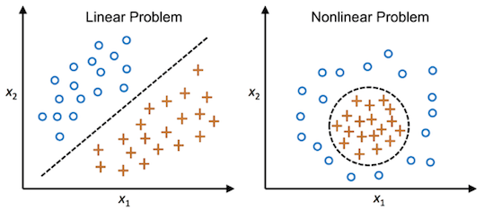
If you wonder what is linearly separable, Python Machine Learning book that we reviewed recently has a nice picture that illustrates it. Assuming we know the data data is generated two groups, when the data is linearly separable, we can easily separate the data in low dimension with a line as shown below. However, when the data is non-linear, we may need a more complex polynomial function to separate the data. Since regular PCA is simply computes PCs as linear combination of the underlying structure in the data, regular PCA will not be able to separate the nonlinear data.
So what will happen if you apply regular PCA to a dataset that is not linearly separable? And how can we deal with such dataset? In this post we will address these questions using sklearn with examples.
Let us get started by loading all the packages needed to illustrate the use of kernal PCA. We will first use sklearn’s datasets module to create non-linear data sets. And then we will load the two modules that will be useful for performing regular PCA and kernal PCA from sklearn.
from sklearn.datasets import make_circles
from sklearn.decomposition import PCA, KernelPCA
import matplotlib.pyplot as plt
import numpy as np
import seaborn as sns
import pandas as pd
To create non-linear data, we will use make_circles() function to create circular data from two groups. Here we generate 200 data paints from two groups, where one group has circular patter and the other random numbers concentrated at the center of the circle. make_circles() function provides the data and the group assignment for each observation.
# Let us create linearly inseparable data
X, y = make_circles(n_samples=200, random_state=1, noise=0.1, factor=0.1)
We will store the data into Pandas dataframe with the group assignment variable.
df =pd.DataFrame(X)
df.columns=['a','b']
df["y"]=y
We can use Seaborn’s scatterplot function to visualize the non-linearity of the data.
sns.scatterplot(data=df,x='a',y='b', hue="y")
As expected, we can see that we have data from two groups with a clear non-linear pattern, in this example circle.


Regular PCA to Non-linear Data
Let us apply regular PCA to this non-learn data and see how the PCs look like. We use sklearn’s PCA function to do the PCA.
scikit_pca = PCA(n_components=2)
X_pca = scikit_pca.fit_transform(X)
To visualize the results from regular PCA, let us make a scatter plot between PC1 and PC2. First, let us store the PCA results into a Pandas dataframe with the known group assignment.
pc_res = pd.DataFrame(X_pca)
pc_res.columns=["pc1","pc2"]
pc_res.head()
pc_res['y']=y
The PCA plot shows that it looks very much like the original data and there is no line that can separate data from two groups.
sns.scatterplot(data=pc_res,x='pc1',y='pc2',hue="y")

Dimensionality Reduction with Kernel PCA using scikit-learn
Now, let us use the same data, but this time apply kernal PCA using kernalPCA() function in sklearn. The basic idea behind kernal PCA is that we use kernal function to project the non-linear data into higher dimensional space where the groups are linearly separable. And then use regular PCA to do the dimentionality reduction.
Here use KernelPCA() function with “rbf” kernel function to perform kernel PCA.
kpca = KernelPCA(kernel="rbf",
                 fit_inverse_transform=True,
                 gamma=10,
                n_components=2)
X_kpca = kpca.fit_transform(X)
Let us save the results into a dataframe as before.
kpca_res = pd.DataFrame(X_kpca)
kpca_res.columns=["kpc1","kpc2"]
kpca_res['y']=y
kpca_res.head()
Now, we can visualize the PCs from kernel PCA using scatter plot and we can clearly see that the data is linearly separable.
sns.scatterplot(data=kpca_res,x='kpc1',y='kpc2', hue="y")


