The high level problem is pretty simple and it goes something like this. You have a dataframe and want to groupby more than one variables, compute some summarized statistics using the remaining variables and use them to do some analysis. Typically plotting something really quick. You can easily imagine a number of variants of this problems. One of the pain points for me is lack of full understanding multi-indexing operations that Pandas enables. So far I have skipped dealing with multi-indexes and do not see myself confronting anytime soon :-). Along the way I have discovered the use of Pandas’ unstack() function multiple times. It is useful for pivot like operation.
Let us work through an example of this with gapminder dataset.
# load pandas
import pandas as pd
import seaborn as sns
import matplotlib.pyplot as plt
We will load gapminder dataset directly from github page.
p2data = "https://raw.githubusercontent.com/cmdlinetips/data/master/gapminder-FiveYearData.csv"
gapminder=pd.read_csv(p2data)
gapminder.head()
country	year	pop	continent	lifeExp	gdpPercap
0	Afghanistan	1952	8425333.0	Asia	28.801	779.445314
1	Afghanistan	1957	9240934.0	Asia	30.332	820.853030
2	Afghanistan	1962	10267083.0	Asia	31.997	853.100710
3	Afghanistan	1967	11537966.0	Asia	34.020	836.197138
4	Afghanistan	1972	13079460.0	Asia	36.088	739.981106
Pandas groupby() on multiple variables
Let us groupby two variables and perform computing mean values for the rest of the numerical variables.
gapminder.groupby(["continent","year"])
<pandas.core.groupby.generic.DataFrameGroupBy object at 0x1a204ecf10>
One of the ways to compute mean values for remaining variables is to use mean() function directly on the grouped object.
df = gapminder.groupby(["continent","year"]).mean().head()
df.head()
When we perform groupby() operation with multiple variables, we get a dataframe with multiple indices as shown below. We have two indices followed by three columns with average values, but with the original column names.


We can use the columns to get the column names. Note that it gives three column names, not the first two index names.
df.columns
Index(['pop', 'lifeExp', 'gdpPercap'], dtype='object')
Pandas reset_index() to convert Multi-Index to Columns
We can simplify the multi-index dataframe using reset_index() function in Pandas. By default, Pandas reset_index() converts the indices to columns.
df.reset_index()
	continent	year	pop	lifeExp	gdpPercap
0	Africa	1952	4.570010e+06	39.135500	1252.572466
1	Africa	1957	5.093033e+06	41.266346	1385.236062
2	Africa	1962	5.702247e+06	43.319442	1598.078825
3	Africa	1967	6.447875e+06	45.334538	2050.363801
4	Africa	1972	7.305376e+06	47.450942	2339.615674
Pandas agg() function to summarize grouped data
Now the simple dataframe is ready for further downstream analysis. One nagging issue is that using mean() function on grouped dataframe has the same column names. Although now we have mean values of the three columns. One can manually change the column names. Another option is to use Pandas agg() function instead of mean().
With agg() function, we need to specify the variable we need to do summary operation. In this example, we have three variables and we want to compute mean. We can specify that as a dictionary to agg() function.
df =gapminder.groupby(["continent","year"]).agg({'pop': ["mean"], 'lifeExp': ["mean"],'gdpPercap':['mean'] })
df.head()
Now we get mean population, life expectancy, gdpPercap for each year and continent. We again get a multi-indexed dataframe with continent and year as indices and three columns. And it looks like this.


Accessing Column Names and Index names from Multi-Index Dataframe
Let us check the column names of the resulting dataframe. Now we get a MultiIndex names as a list of tuples. Each tuple gives us the original column name and the name of aggregation operation we did. In this example, we used mean. It can be other summary operations as well.
df.columns
MultiIndex([(      'pop', 'mean'),
            (  'lifeExp', 'mean'),
            ('gdpPercap', 'mean')],
           )
The column names/information are in two levels. We can access the values in each level using Pandas’ get_level_values() function.
With columns.get_level_values(0), we get the column names.
df.columns.get_level_values(0)
Index(['pop', 'lifeExp', 'gdpPercap'], dtype='object')
With get_level_values(1), we get the second level of column names, which is the aggregation function we used.
df.columns.get_level_values(1)
Index(['mean', 'mean', 'mean'], dtype='object')
Similarly, we can also get the index values using index.get_level_values() function. Here we get the values of the first index.
df.index.get_level_values(0)
Index(['Africa', 'Africa', 'Africa', 'Africa', 'Africa', 'Africa', 'Africa',
       'Africa', 'Africa', 'Africa', 'Africa', 'Africa', 'Americas',
       'Americas', 'Americas', 'Americas', 'Americas', 'Americas', 'Americas',
       'Americas', 'Americas', 'Americas', 'Americas', 'Americas', 'Asia',
       'Asia', 'Asia', 'Asia', 'Asia', 'Asia', 'Asia', 'Asia', 'Asia', 'Asia',
       'Asia', 'Asia', 'Europe', 'Europe', 'Europe', 'Europe', 'Europe',
       'Europe', 'Europe', 'Europe', 'Europe', 'Europe', 'Europe', 'Europe',
       'Oceania', 'Oceania', 'Oceania', 'Oceania', 'Oceania', 'Oceania',
       'Oceania', 'Oceania', 'Oceania', 'Oceania', 'Oceania', 'Oceania'],
      dtype='object', name='continent')
similarly, we can get the values of second index using index.get_level_values(1).
df.index.get_level_values(1)
Int64Index([1952, 1957, 1962, 1967, 1972, 1977, 1982, 1987, 1992, 1997, 2002,
            2007, 1952, 1957, 1962, 1967, 1972, 1977, 1982, 1987, 1992, 1997,
            2002, 2007, 1952, 1957, 1962, 1967, 1972, 1977, 1982, 1987, 1992,
            1997, 2002, 2007, 1952, 1957, 1962, 1967, 1972, 1977, 1982, 1987,
            1992, 1997, 2002, 2007, 1952, 1957, 1962, 1967, 1972, 1977, 1982,
            1987, 1992, 1997, 2002, 2007],
           dtype='int64', name='year')
Fixing Column names after Pandas agg() function to summarize grouped data
Since we have both the variable name and the operation performed in two rows in the Multi-Index dataframe, we can use that and name our new columns correctly.
Here we combine them to create new column names using Pandas map() function.
df.columns.map('_'.join)
Index(['pop_mean', 'lifeExp_mean', 'gdpPercap_mean'], dtype='object')
We can change the column names of the dataframe.
df.columns=df.columns.map('_'.join)
df.head()
And now we have summarized dataframe with correct names. Using agg() function to summarize takes few more lines, but with right column names, when compared to Pandas’ mean() function.


The resulting dataframe is still Multi-Indexed and we can use reset_index() function to convert the row index or rownames as columns as before.
And we get a simple dataframe with right column names.
df=df.reset_index()
df.head()

continent	year	pop_mean	lifeExp_mean	gdpPercap_mean
0	Africa	1952	4.570010e+06	39.135500	1252.572466
1	Africa	1957	5.093033e+06	41.266346	1385.236062
2	Africa	1962	5.702247e+06	43.319442	1598.078825
3	Africa	1967	6.447875e+06	45.334538	2050.363801
4	Africa	1972	7.305376e+06	47.450942	2339.615674
Grouped Line Plots with Seaborn’s lineplot
In the above example, we computed summarized values for multiple columns. Typically, one might be interested in summary value of a single column, and making some visualization using the index variables. Let us take the approach that is similar to above example using agg() function.
In this example, we use single variable for computing summarized/aggregated values. Here we compute median life expectancy for each year and continent. We also create new appropriate column name as above.
df =gapminder.groupby(["continent","year"]).
              agg({'lifeExp': ["median"] })
df.columns=df.columns.map('_'.join)
df=df.reset_index()
df.head()
	continent	year	lifeExp_median
0	Africa	1952	38.8330
1	Africa	1957	40.5925
2	Africa	1962	42.6305
3	Africa	1967	44.6985
4	Africa	1972	47.0315
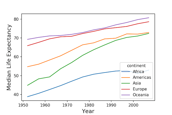
Note that, our resulting data is in tidy form and we can use Seaborn’s lineplot to make grouped line plots of median life expectancy over time for 5 continents.
plt.figure(figsize=(8,6))
sns.lineplot(x='year', y='lifeExp_median', hue="continent", data=df)
plt.xlabel("Year", size=14)
plt.ylabel("Median Life Expectancy", size=14)
plt.savefig("Multi_group_line_plot_Seaborn.png",
                    format='png',
                    dpi=150)
We get nice multiple lineplots with Seaborn.


Pandas unstack function to get data in wide form
For some reason, if you don’t want the resulting data to be in tidy form, we can use unstack() function after computing the summarized values.
Here we use Pandas’ unstack() function after computing median lifeExp for each group. And we get our data in wide form. When you groupby multiple variables, by default the last level will be on the rows in the wide form.
gapminder.groupby(["year","continent"])['lifeExp'].median().unstack().head()
continent	Africa	Americas	Asia	Europe	Oceania
year
1952	38.8330	54.745	44.869	65.900	69.255
1957	40.5925	56.074	48.284	67.650	70.295
1962	42.6305	58.299	49.325	69.525	71.085
1967	44.6985	60.523	53.655	70.610	71.310
1972	47.0315	63.441	56.950	70.885	71.910
If we want wide form data, but with different variable on column, we can specify the level or variable name to unstack() function. For example, to get year on columns, we would use unstack(“year”) as shown below.
gapminder.groupby(["year","continent"])['lifeExp'].median().unstack("year").head()

year	1952	1957	1962	1967	1972	1977	1982	1987	1992	1997	2002	2007
continent
Africa	38.833	40.5925	42.6305	44.6985	47.0315	49.2725	50.756	51.6395	52.429	52.759	51.2355	52.9265
Americas	54.745	56.0740	58.2990	60.5230	63.4410	66.3530	67.405	69.4980	69.862	72.146	72.0470	72.8990
Asia	44.869	48.2840	49.3250	53.6550	56.9500	60.7650	63.739	66.2950	68.690	70.265	71.0280	72.3960
Europe	65.900	67.6500	69.5250	70.6100	70.8850	72.3350	73.490	74.8150	75.451	76.116	77.5365	78.6085
Oceania	69.255	70.2950	71.0850	71.3100	71.9100	72.8550	74.290	75.3200	76.945	78.190	79.7400	80.7195
One of the advantages with using unstack() is that we have sidestepped the multi-index to simple index and we can quickly make exploratory data visualization with different variables. In this example below, we make a line plot again between year and median lifeExp for each continent. However this time we simply use Pandas’ plot function by chaining the plot() function to the results from unstack().
gapminder.groupby(["year","continent"])['lifeExp'].median().unstack().plot()
And we get almost similar plot as before, since Pandas’ plot function calls Matplotlib under the hood.